New Spreadsheet Features: Freeze Rows and Conditional Formatting
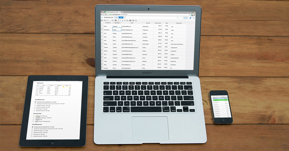
We're adding a bunch of new features to Quip Spreadsheets based on your feedback. Last month, we released @-mentions and images in cells, keyboard shortcuts, and improved mobile selection. Today, we're releasing freezing rows, conditional formatting, and table mode.
Freeze Rows
One of the most requested features for Spreadsheets has been the ability to freeze rows. In big spreadsheets, it's essential to be able to reference column headers and context at the top of the spreadsheet as you scroll through the data. Now you can freeze as many rows as you want with the click of your mouse:
And don't worry — freezing columns is next on our list!
Conditional Formatting
With conditional formatting, you can highlight cells based on rules you define. This can help you visualize patterns and trends in a dataset that would otherwise be difficult to parse in a sea of numbers. We've added basic rules for string and numerical comparison, and we plan on adding more rules over time. Send us feedback if you think we've missed any important ones.
To apply conditional formatting to your spreadsheet, click the formatting icon in the menu above your sheet:
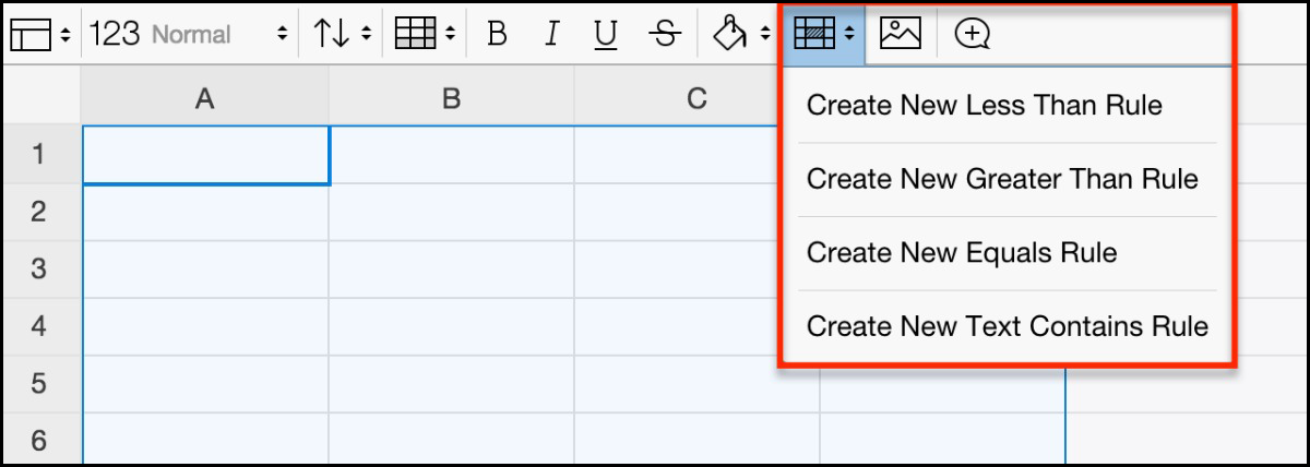
You can create rules using the dropdown. In the example below, conditional formatting is used to highlight scores from a test:
Table Mode
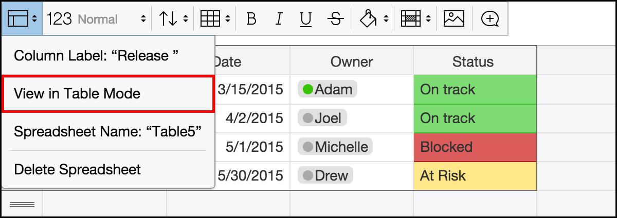
Spreadsheets in Quip can be standalone workbooks or embedded in a document. With table mode, you can embed a visually simplified spreadsheet in a document without the additional complexity of row and column numbers.
To hide row and column numbers in your spreadsheet, select “View in Table Mode” in the settings menu above your sheet.
We Love Feedback
We're always improving Quip based on your feedback. If you have ideas for new features or how to make Quip work better for you and your team, drop us a line.